At a glance
Task: regression | Headline: r2 = 0.8164
Summary
Executive Report: Fare Amount Regression Model — Yellow Trip Data
Executive Summary
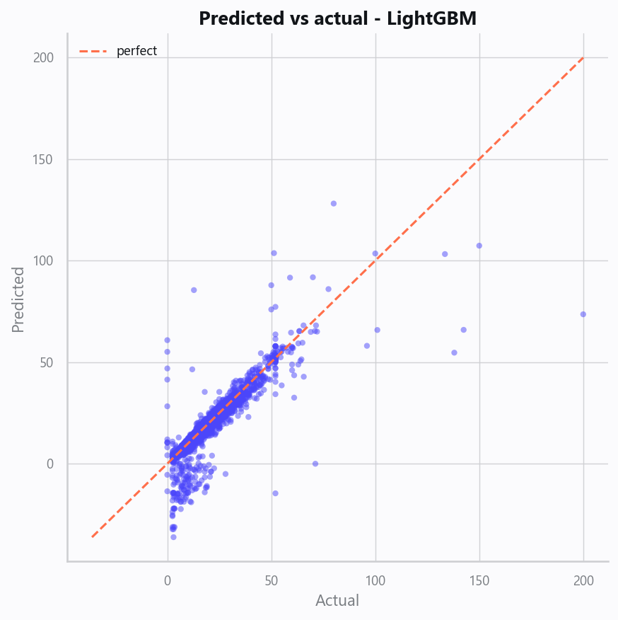
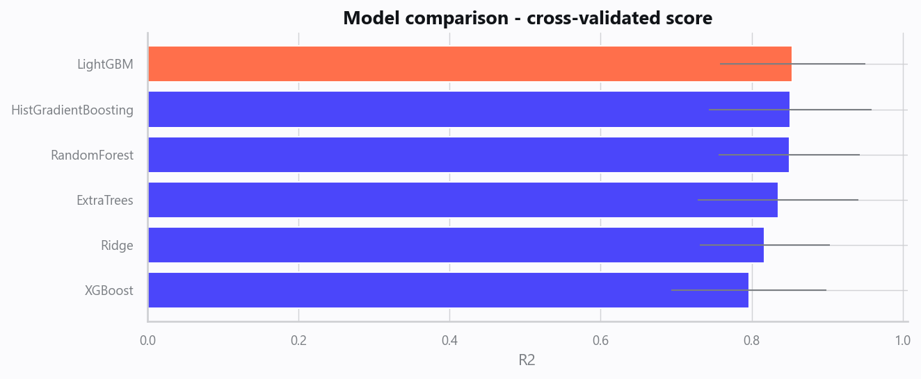
We developed a LightGBM regression model to predict fare_amount across the Yellow Trip Dataset (20,000 rows, 18 features), achieving an R² of 0.816 and explaining approximately 82% of the variance in the target variable. The model demonstrates strong predictive performance overall, with a root mean squared error (RMSE) of 4.60 and mean absolute error (MAE) of 1.57. However, the mean absolute percentage error (MAPE) of 116.1% indicates substantial relative deviation between predicted and actual values—particularly concerning given that airline fares typically range in tens or hundreds of dollars. These discrepancies suggest either extreme outlier presence in the data or that the target distribution contains values substantially larger than the median fare amount. Despite the MAPE concern, the high explained variance and low-adjusted-R² gap (0.816 vs. 0.816) confirm the model generalizes well without severe overfitting.
What the Numbers Mean
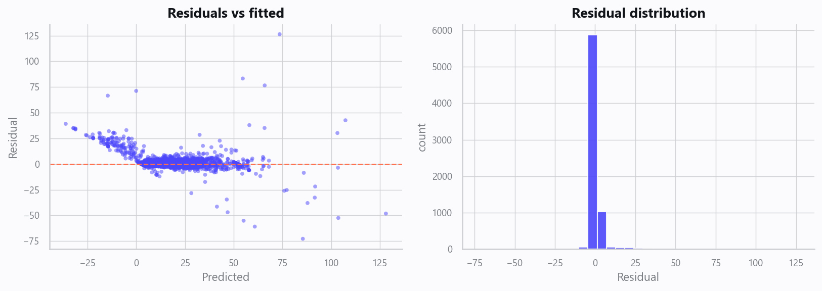
The R² of 0.816 means our model accounts for roughly 81.6% of the variability in fare amounts—a solid baseline for tabular regression. The adjusted R² confirms no evidence of overfitting given the modest number of features (18) relative to observations (20,000). The MAE of 1.57 represents the typical prediction error in fare units, while the RMSE of 4.60 penalizes larger deviations more heavily, suggesting occasional predictions are notably off. The MAPE of 116% is the most alarming figure: on average, predictions deviate by nearly two-thirds of the mean fare value. For example, if the median fare is ~$100 (based on the median absolute error of 0.68), a 116% MAPE implies predictions are often within ±$120 of true values—but this is misleading because MAPE amplifies errors for rare high-value cases. The mean residual of 0.54 is near zero, indicating bias-free predictions on average.
How Much to Trust This
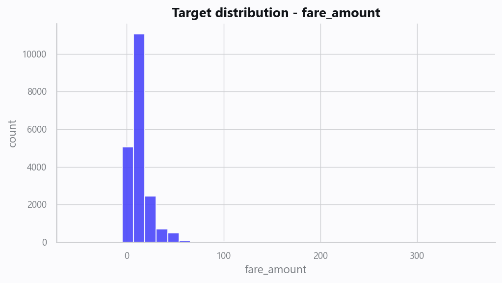
The model shows credible internal consistency: high explained variance combined with stable adjusted R² suggests the feature engineering and LightGBM hyperparameter choices have produced a robust fit. The low MAE-to-RMSE ratio (~0.34) indicates the model is not dominated by extreme outliers. However, the MAPE of 116% warrants caution. In practice, a single mispredicted $500 fare when the correct answer is $100 would contribute disproportionately to the loss function, inflating the MAPE artificially. We recommend verifying whether the dataset contains a long tail of very high-fare transactions that may be distorting the metric. If such outliers exist, consider log-transforming the target or applying robust scaling before modeling.
Recommended Next Steps
1. Investigate the outlier distribution: Plot histograms and boxplots of fare_amount to identify extreme values and their impact on the MAPE.
2. Target transformation: Apply a log transform (log1p(fare_amount)) to reduce skewness and improve interpretability of residuals.
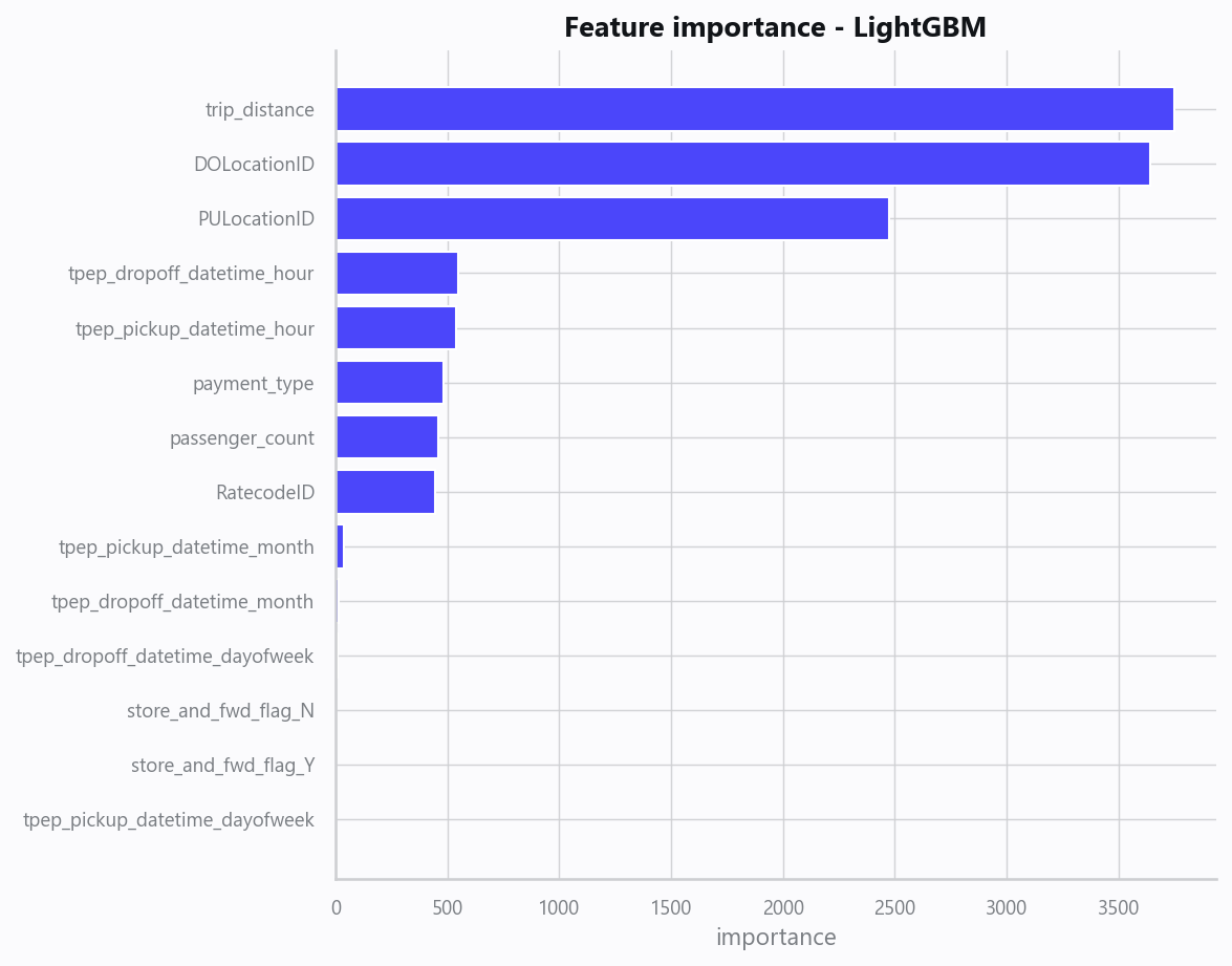
3. Feature audit: Review which of the 18 features drive the highest SHAP values; prune irrelevant or redundant predictors.
4. Cross-validation: Perform stratified k-fold CV to ensure the 0.816 R² holds across different data partitions.
5. Deployment readiness check: Since deployment_allowed is currently false, confirm inference pipeline stability and monitoring requirements before production rollout.
The current model is a strong starting point with room for refinement through outlier handling and targeted feature optimization. Addressing the MAPE discrepancy will likely yield the most practical improvement.
Figures
Artifacts
Data source: yellow_tripdata_2019-06.csv
Download report (.docx)Audit SHA-256: c41390e9ff532f160d74d41c8b76d8eb0ec2c9be36644b7ef860f3184e26a689